More search.
The same decisions.
The MC-taught linear bot now runs substantially faster. Fixed-work comparisons preserve every sampled result and recommendation. All intensive measurements ran inside a Linux ARM container limited to two CPU cores and 2 GiB RAM, with no swap.
1 worker · 5 repeats
2 workers · 3 repeats
2 simultaneous clients
32 fresh regression deals
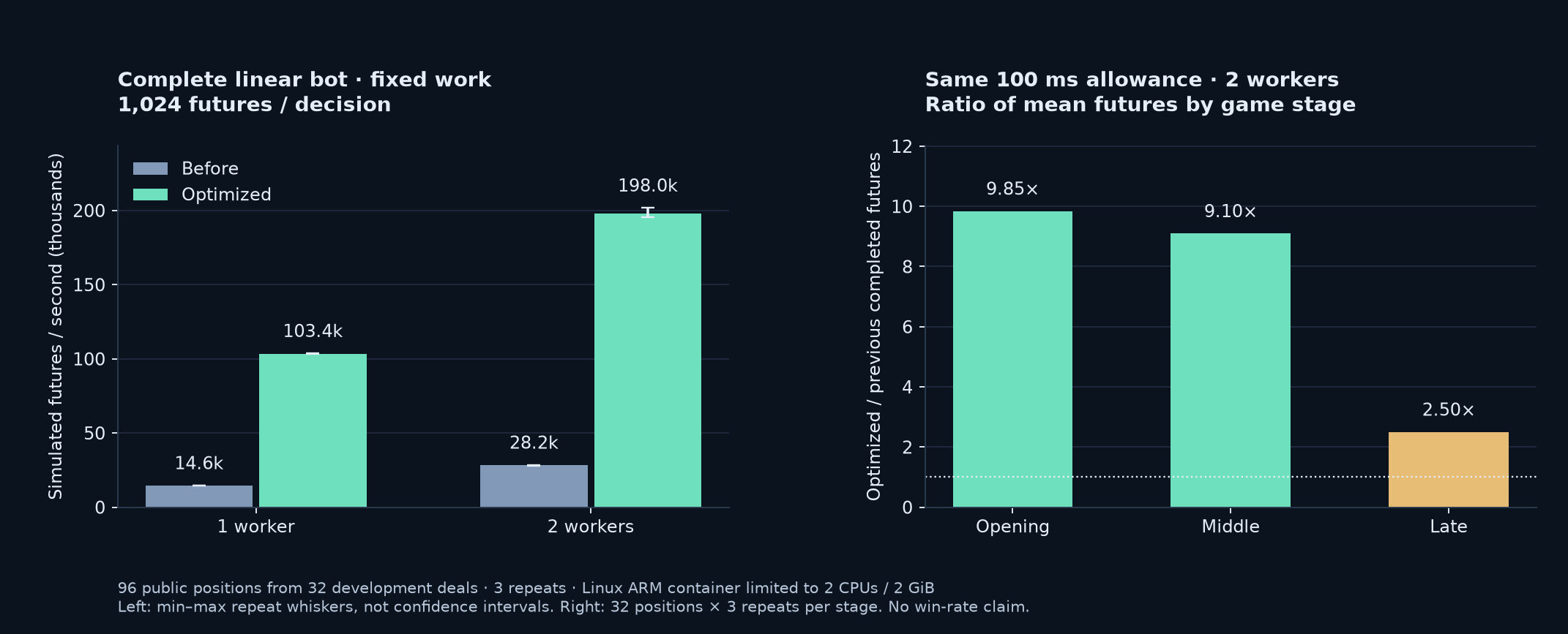
On small screens, scroll the chart or tables sideways. Whiskers show observed repeat ranges, not statistical confidence intervals.
What the measurements include
The native comparison includes the JSON boundary and precomputed linear priors. The complete-bot comparison also includes public feature calculation, linear inference, recommendation explanations, worker communication, and batch scheduling. Immediate-win shortcuts were disabled in these position benchmarks so both versions had to simulate; normal play still uses those shortcuts. Each version handles the same 96 positions × 3 repeats × 1,024 futures below.
| Workers | Version | Futures / second | Mean decision (ms) | p95 decision (ms) | Decisions |
|---|---|---|---|---|---|
| 1 | Before | 14,619 | 69.95 | 144.67 | 288 |
| 1 | Optimized | 103,395 | 9.82 | 18.52 | 288 |
| 2 | Before | 28,244 | 71.61 | 148.67 | 288 |
| 2 | Optimized | 198,031 | 10.02 | 19.16 | 288 |
Throughput uses total futures divided by batch wall time. Decision latency uses individual calls; two workers improve aggregate capacity, not the latency of a single search. Each search remains single-threaded.
What fits in 100 ms?
With two workers, the optimized bot completed 2.78× as many futures overall. The median gain across individual positions was 9.32×. Both are useful: easy late positions contribute far more futures to the aggregate count, while openings and middle games benefit more from cheaper move scoring.
| Stage | Before: mean futures | Optimized: mean futures | Ratio |
|---|---|---|---|
| Opening | 723 | 7,122 | 9.85× |
| Middle | 1,744 | 15,872 | 9.10× |
| Late | 58,344 | 146,018 | 2.50× |
The stages are the first, middle, and last recorded position from each collected game. Last snapshots have 5–11 defeated enemies (median 10), and can precede either a win or a loss. Each stage contains 32 positions, repeated three times per version. The simulation cap was raised to 1,000,000 solely to keep it from ending these timed searches; no call reached it. The final bot’s two-worker p95 was 104.33 ms: the allowance is checked between futures, and serialization/explanations add a small overhead.
This is a speed study. More futures do not establish a higher win rate. The corpus comes from development/training deals, not held-out strength evaluation. Repeated positions are not independent games. These are host-CPU measurements in a constrained ARM Linux container, not measurements on the deployment box.
Where the work disappeared
The initial instruction profile was dominated by legal-move construction and allocation/free operations. The same profiling workload fell from 17.07 billion to 1.99 billion instructions (88.4% fewer). Callgrind counts instructions; these percentages are not CPU-time shares.
- Borrow public state. Avoid cloning entire observations and belief vectors for each simulated move.
- Visit legal moves on the stack. Generate combinations directly; consider payments without allocating a card vector for every candidate.
- Sort once per hand. Preserve canonical card order and exact tie breaks without sorting every subset.
- Reuse defensive sums. Share partial card-cost sums while preserving the original floating-point addition order.
- Keep cached moves inline. Use a bounded cache with compact moves and a lightweight private hash; no heap allocation per cache hit.
- Prepare and reuse sampled worlds. Prepare public constraints once, sample fresh consistent worlds, and reuse their storage.
- Omit unused belief updates. Full heuristic continuations use public card counts. Their physical rules and chance stream stay identical; tree search keeps belief tracking.
- Inline hot scoring. Let the compiler combine scoring and effects with the selection loop. The learned weights and rollout policy stay unchanged.
Experiments we did not keep
Collapsing additional defensive cache keys showed no clear speed gain. A 65,536-entry cache was slower than the existing 16,384-entry default on the tested 4,096-future workload; 2,048 entries performed about the same. Fat LTO did not beat thin LTO. These trials and their exact outputs are retained in the experiment folder.
Correctness and resource checks
- 60 Python tests and 7 Rust tests passed. Coverage includes official-rule edge cases, observation boundaries, seeded randomness, exhaustive legal-subset comparisons, and identical physical transitions with and without continuation belief bookkeeping.
- 32 fresh deals, 1,838 decisions: full recommendations and replay logs matched the frozen pre-optimization bot at a fixed 128-future cap. This is regression evidence, not a win-rate experiment.
- Two-client HTTP stress test: ten one-second hints, peak RSS 31.0 MiB, with zero rollout truncations. RSS is process memory, not the whole operating system.
- Container lifetime peak: 862 MiB including build/profiling work and file cache; no memory-limit or OOM events. This is separate from the server RSS measurement.
- Deployment safeguards: two simultaneous searches, no unbounded search queue, evaluation pools capped at two workers; systemd template caps CPU at two cores and app memory at 1.5 GiB, leaving headroom on a 2 GiB machine. Cloud deployment was not changed.
Remaining limits
This is not proof that further optimization is impossible. Candidate scoring and legal-subset traversal still dominate the hot loop. The next defensible step is profiling the actual deployment CPU and checking a broader state distribution. Parallelizing one adaptive search or changing rollout policies would be a separate algorithm experiment, requiring new strength comparisons.
Reproduce and inspect the evidence
The frozen binaries, model, public positions, source snapshots, raw timings, profiles, regression replays, and rejected trials are in experiments/linear-optimization/. See docs/NATIVE.md for constrained-container commands.
Download audited summary and source hashes ↓
python3 tools/compare_linear.py --libraries '{"before":"experiments/linear-optimization/baseline.so","optimized":"experiments/linear-optimization/final.so"}' --repeat 5 --output /tmp/native-repeat.json
python3 tools/bench_linear_full.py --libraries '{"before":"experiments/linear-optimization/baseline.so","optimized":"experiments/linear-optimization/final.so"}' --workers 2 --repeat 3 --output /tmp/full-repeat.json
Run the Linux binaries inside the documented container; do not load them into macOS Python. The normal app uses a separately rebuilt native library for your operating system.
Model SHA-256: dc1c0b485eb7ec14cab5…
Source fingerprint: 0595762fade80e7dec57…